In this example we consider the ZelazoKolb1972 dataset, which is
built-in restriktor. The data consist of ages in months at which an child starts
to walk for four treatment groups. The first treatment group (Active) received a
special walking exercise for 12 minutes per day beginning at age 1 week and
lasting 7 weeks. The second group (Passive) received daily exercises but not
the special walking exercises. The third group (Control) is the control; they did
not receive any exercises or other treatments. The fourth group (No) of children
were checked weakly for progress but they did not receive any special exercises.
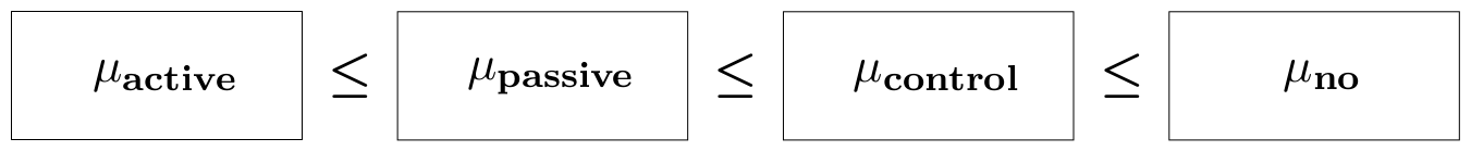
The purpose of the study was to test the claim that the walking exercises are associated with a reduction in the mean age at which children start to walk. Then, the order-constrained hypothesis can be formulated as: $$ H_1: \mu_1 \leq \mu_2 \leq \mu_3 \leq \mu_4, $$ where $ \mu_j $ is the population mean for group $j$. A graphical representation is shown below.
In what follows, we describe all steps to test this order constrained hypothesis.
library(restriktor)
The ZelazoKolb1972 dataset is available in restriktor and can be
called directly, see next step.
An ANOVA model is just a special case of the linear model. Therefore, we can make
use of the built-in linear model lm() function in R. The intercept (-1)
is removed, such that the regression coefficients reflect the group means. To fit
the unrestricted linear model type
fit.ANOVA <- lm(Age ~ -1 + Group, data = ZelazoKolb1972)
The constraint syntax can be constructed by using the factor level names preceded by the factor name. To get the correct names, type
names(coef(fit.ANOVA))
[1] "GroupActive" "GroupControl" "GroupNo" "GroupPassive"
Based on these factor level names, we can construct the constraint syntax:
myConstraints <- ' GroupActive < GroupPassive < GroupControl < GroupNo '

# note that the constraint syntax is enclosed within single quotes.
The restricted ANOVA model is estimated using the restriktor() function. The first argument to restriktor() is the fitted linear model and the second argument is the constraint syntax.
restr.ANOVA <- restriktor(fit.ANOVA, constraints = myConstraints)
summary(restr.ANOVA)
Call:
conLM.lm(object = fit.ANOVA, constraints = myConstraints)

Restriktor: restricted linear model:

Residuals:
    Min      1Q  Median      3Q     Max
-2.7083 -0.8500 -0.3500  0.6375  3.6250

Coefficients:
             Estimate Std. Error t value  Pr(>|t|)
GroupActive  10.12500    0.61907  16.355 1.191e-12 ***
GroupControl 11.70833    0.61907  18.913 8.774e-14 ***
GroupNo      12.35000    0.67815  18.211 1.736e-13 ***
GroupPassive 11.37500    0.61907  18.375 1.478e-13 ***
---
Signif. codes:  0 '***' 0.001 '**' 0.01 '*' 0.05 '.' 0.1 ' ' 1

Residual standard error: 1.5164 on 19 degrees of freedom
Standard errors: standard
Multiple R-squared remains 0.986

Generalized Order-Restricted Information Criterion:
 Loglik Penalty   Goric
-40.014   3.098  86.224
## by default the iht() function prints a summary of all available
## hypothesis tests. A more detailed overview of the separate hypothesis
## tests can be requested by specifying the test = "" argument, e.g.,
## iht(restr.ANOVA, test = "A").
iht(fit.ANOVA, constraints = myConstraints)
Restriktor: restricted hypothesis tests ( 19 residual degrees of freedom ):


Multiple R-squared remains 0.986

Constraint matrix:
   GroupActive GroupControl GroupNo GroupPassive    op rhs active
1:          -1            0       0            1    >=   0     no
2:           0            1       0           -1    >=   0     no
3:           0           -1       1            0    >=   0     no


Overview of all available hypothesis tests:

Global test: H0: all parameters are restricted to be equal (==)
         vs. HA: at least one inequality restriction is strictly true (>)
       Test statistic: 6.4267,   p-value: 0.03085

Type A test: H0: all restrictions are equalities (==)
         vs. HA: at least one inequality restriction is strictly true (>)
       Test statistic: 6.4267,   p-value: 0.03085

Type B test: H0: all restrictions hold in the population
         vs. HA: at least one restriction is violated
       Test statistic: 0.0000,   p-value: 1

Type C test: H0: at least one restriction is false or active (==)
         vs. HA: all restrictions are strictly true (>)
       Test statistic: 0.3807,   p-value: 0.3538

Note: Type C test is based on a t-distribution (one-sided),
      all other tests are based on a mixture of F-distributions.
The results provide affirmative evidence in favor of the informative hypothesis. Hypothesis test Type B is not rejected ($\bar{\text{F}}^{\text{B}}_{(0,1,2,3; 19)}$ = 0, p = 1) in favor of the unconstrained hypothesis (i.e., best fitting hypothesis). This means that the constraints are in line with the data. Hypothesis test Type A is rejected in favor of the order-constrained hypothesis ($\bar{\text{F}}^{\text{A}}_{(0,1,2,3; 19)}$, p = .03085). We can conclude that the walking exercises are associated with a reduction in the mean age at which children start to walk.