In this example we consider the AngerManagement dataset, which is
built-in restriktor. The data consists of a persons' decrease in aggression level
between week 1 (intake) and week 8 (end of training) for four different treatment
groups of anger management training, namely (1) no training, (2) physical training,
(3) behavioral therapy, and (4) a combination of physical exercise and behavioral
therapy. In addition, the dataset includes the covariate age. The purpose of the
study was to test the assumption that the exercises would be associated with a
reduction in the mean aggression levels with respect to the covariate age. In
particular, the hypothesis of interest is:
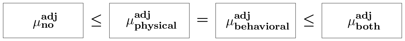
$$ H^{adj}_1: \mu^{adj}_{No} \leq \big[\mu^{adj}_{Physical} = \mu^{adj}_{behavioral}\big] \leq \mu^{adj}_{Both}, $$
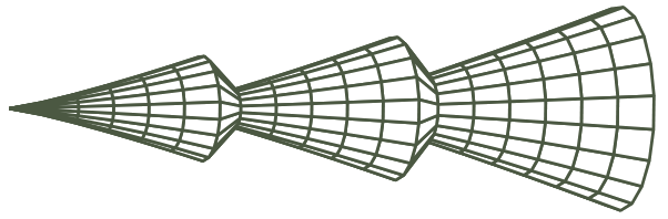
where $\mu^{adj}_j$ denotes the population adjusted mean for group $j$. This hypothesis states that the decrease in aggression levels is smallest for the 'no training' group, larger for the 'physical training' group and “behavioral therapy' group, with no preference for either method, and largest in the 'combination of physical exercise and behavioral therapy' group. Below a graphical representation of the order-constrained hypothesis.
In what follows, we describe all steps to test this hypothesis.
library(restriktor)
The AngerManagement dataset is available in restriktor and can be
called directly, see next step.
To obtain adjusted means, the easiest way is by creating a new variable where the covariate 'age' is centered at its average. This can be done as follows:
AngerManagement$Age_Z <- AngerManagement$Age - mean(AngerManagement$Age)
We use the newly created variable 'Age_Z' to get mean adjusted estimates:
fit.ANCOVA <- lm(Anger ~ -1 + Group + Age_Z, data = AngerManagement)
The constraint syntax can be constructed by using the factor level names. The correct names can be obtained in R by typing:
names(coef(fit.ANCOVA))
[1] "GroupBehavioral" "GroupBoth"       "GroupNo"         "GroupPhysical"
[5] "Age_Z"
Based on these factor level names, we can construct the constraint syntax:
myConstraints <- ' GroupNo < GroupPhysical = GroupBehavioral < GroupBoth '

#note that the constraint syntax is enclosed within single quotes.
The restriktor() function computes the restricted estimates. The first argument to restriktor() is the fitted linear model and the second argument is the constraint syntax.
restr.ANCOVA <- restriktor(fit.ANCOVA, constraints = myConstraints)
summary(restr.ANCOVA)
Call:
conLM.lm(object = fit.ANCOVA, constraints = myConstraints)

Restriktor: restricted linear model:

Residuals:
     Min       1Q   Median       3Q      Max
-3.12596 -1.34314 -0.06718  1.23245  5.05649

Coefficients:
                 Estimate Std. Error t value  Pr(>|t|)
GroupBehavioral  1.951082   0.467593  4.1726 0.0001889 ***
GroupBoth        4.068634   0.702820  5.7890 1.465e-06 ***
GroupNo         -0.170797   0.697417 -0.2449 0.8079643
GroupPhysical    1.951082   0.467593  4.1726 0.0001889 ***
Age_Z            0.021632   0.164371  0.1316 0.8960526
---
Signif. codes:  0 '***' 0.001 '**' 0.01 '*' 0.05 '.' 0.1 ' ' 1

Residual standard error: 2.0908 on 35 degrees of freedom
Standard errors: standard
Multiple R-squared reduced from 0.685 to 0.609

Generalized Order-Restricted Information Criterion:
  Loglik  Penalty    Goric
-84.1525   3.9248 176.1546
## by default the iht() function prints a summary of all available
## hypothesis tests. A more detailed overview of the separate hypothesis
## tests can be requested by specifying the test = "" argument, e.g.,
## iht(restr.ANCOVA, test = "A").
iht(fit.ANCOVA, constraints = myConstraints)
Restriktor: restricted hypothesis tests ( 35 residual degrees of freedom ):

Multiple R-squared reduced from 0.685 to 0.609

Constraint matrix:
   GroupBehavioral GroupBoth GroupNo GroupPhysical Age_Z    op rhs active
1:              -1         0       0             1     0    ==   0    yes
2:               0         0      -1             1     0    >=   0     no
3:              -1         1       0             0     0    >=   0     no


Overview of all available hypothesis tests:

Global test: H0: all parameters are restricted to be equal (==)
         vs. HA: at least one inequality restriction is strictly true (>)
       Test statistic: 44.5941,   p-value: <0.0001

Type A test: H0: all restrictions are equalities (==)
         vs. HA: at least one inequality restriction is strictly true (>)
       Test statistic: 19.9963,   p-value: 0.0001172

Type B test: H0: all restrictions hold in the population
         vs. HA: at least one restriction is violated
       Test statistic: 8.4966,   p-value: 0.02751

Note: All tests are based on a mixture of F-distributions
      (Type C test is not applicable because of equality restrictions.)
The results do NOT provide evidence in favor of the informative hypothesis. Hypothesis test Type B is rejected ($\bar{\text{F}}^{\text{B}}_{(1,2,3; 35)}$ = 8.50, p = .03) in favor of the unconstrained (i.e., best fitting) hypothesis. This means that the order constraints are not in line with the data. Although, evaluating hypothesis test Type A is redundant if hypothesis test Type B is rejected, its results ($\bar{\text{F}}^{\text{A}}_{(0,1,2; 35)}$ = 19.99, p = .001) show that the null-hypothesis is rejected in favor of the order-constrained hypothesis. This clearly demonstrates that rejecting hypothesis test Type A does not mean that the alternative (i.e., order-constrained) hypothesis is true. It is only its power that is concentrated in the alternative hypothesis.